Quantities for R – Ready for a CRAN release
This is the fourth blog post on
quantities, an
R-Consortium funded project for quantity calculus with R. It is aimed at
providing integration of the ‘units’ and ‘errors’ packages for a
complete quantity calculus system for R vectors, matrices and arrays,
with automatic propagation, conversion, derivation and simplification of
magnitudes and uncertainties. This article summarises the latest
enhancements and investigates how to fit linear regressions with
quantities. In previous articles, we discussed a first working
prototype,
units and errors
parsing,
and data wrangling operations with
quantities.
Latest enhancements
In the following, we briefly describe some important enhancements made
to the units, errors and quantities packages. Also, we would like
to note that, thanks to Katharine Mullen’s careful review, packages
units, errors and constants are now listed in the ChemPhys CRAN
Task View.
Mixed units
Apart from various minor improvements and bug fixes, the most notable new feature is the support for mixed units, that will be released on CRAN, foreseeably, within a month.
One of the most prominent design decisions made in the units package
(which applies to errors and quantities as well), following R’s
philosophy, is that units objects are fundamentally vectors. This
means that a units (errors, quantities) object represents one or
more measurement values of the same quantity, with the same unit (for
instance, repeated measurements of the same quantity). Thus, different
quantities, with different units, must belong to different objects.
However, Bill Denney raised an interesting use case (#134, #145) in which different quantities need to be manipulated in a single data structure. Very briefly, he receives heterogeneous measurements of different analytes from clinical studies as follows:
(analytes <- data.frame(
  analyte=c("glucose", "insulin", "glucagon"),
  original_unit=c("mg/dL", "IU/L", "mmol/L"),
  original_value=c(1, 2, 3),
  new_unit=c("mmol/L", "mg/dL", "mg/L"),
  stringsAsFactors=FALSE
))
##    analyte original_unit original_value new_unit
## 1  glucose         mg/dL              1   mmol/L
## 2  insulin          IU/L              2    mg/dL
## 3 glucagon        mmol/L              3     mg/L
To be able to convert these values to the new units, first we need to define some conversion constants between grams and IUs (which stands for International Unit) or moles of a particular substance (note: numbers may be wrong):
# some adjustments
(analytes <- within(analytes, {
  for (i in seq_along(analyte)) {
    original_unit[i] <- gsub("(mol|IU)", paste0("\\1_", analyte[i]), original_unit[i])
    new_unit[i] <- gsub("(mol|IU)", paste0("\\1_", analyte[i]), new_unit[i])
  }
  i <- NULL
}))
##    analyte   original_unit original_value       new_unit
## 1  glucose           mg/dL              1 mmol_glucose/L
## 2  insulin    IU_insulin/L              2          mg/dL
## 3 glucagon mmol_glucagon/L              3           mg/L
library(units)
## udunits system database from /usr/share/udunits
install_conversion_constant("mol_glucose", "g", 180.156)
install_conversion_constant("g", "IU_insulin", 25113.32)
install_conversion_constant("mol_glucagon", "g", 3482.80)
Then, the development version of units provides a new method called
mixed_units() intended for this use case:
(analytes <- within(analytes, {
  original_value <- mixed_units(original_value, original_unit)
  new_value <- set_units(original_value, new_unit)
  original_unit <- new_unit <- NULL
}))
##    analyte      original_value                   new_value
## 1  glucose           1 [mg/dL] 0.05550745 [mmol_glucose/L]
## 2  insulin    2 [IU_insulin/L]         0.007963901 [mg/dL]
## 3 glucagon 3 [mmol_glucagon/L]              10448.4 [mg/L]
Mixed units are basically lists with a custom class, and each element of
the list is a units object:
analytes$original_value
## Mixed units: IU_insulin/L (1), mg/dL (1), mmol_glucagon/L (1)
## 1 [mg/dL], 2 [IU_insulin/L], 3 [mmol_glucagon/L]
class(analytes$original_value)
## [1] "mixed_units"
unclass(analytes$original_value)
## [[1]]
## 1 [mg/dL]
##
## [[2]]
## 2 [IU_insulin/L]
##
## [[3]]
## 3 [mmol_glucagon/L]
class(analytes$original_value[[1]])
## [1] "units"
Still, units objects cannot be concatenated into mixed lists unless
explicitly enabled by the user, thus maintaining backwards
compatibility:
c(as_units("m"), as_units("s")) # error, cannot convert, cannot mix
## Error in c.units(as_units("m"), as_units("s")): units are not convertible, and cannot be mixed; try setting units_options(allow_mixed = TRUE)?
c(as_units("m"), as_units("s"), allow_mixed=TRUE)
## Mixed units: m (1), s (1)
## 1 [m], 1 [s]
This behaviour can be controlled also by the global option allow_mixed
(see help(units_options)). Finally, note that mixed units with
non-heterogeneous units are not simplified either unless explicitly
requested:
(x <- mixed_units(1:3, c("m", "s", "m")))
## Mixed units: m (2), s (1)
## 1 [m], 2 [s], 3 [m]
as_units(x) # error, cannot convert, cannot mix
## Error in c.units(structure(1L, units = structure(list(numerator = "m", : units are not convertible, and cannot be mixed; try setting units_options(allow_mixed = TRUE)?
x[c(1, 3)]
## Mixed units: m (2)
## 1 [m], 3 [m]
as_units(x[c(1, 3)])
## Units: [m]
## [1] 1 3
Compatibility with this feature has been also added to the quantities
package. Specifically, lists of mixed units can contain either units
or quantities objects, and additional methods have been defined to
deal with them transparently.
library(quantities)
## Loading required package: errors
c(set_quantities(1, m, 0.1), set_quantities(2, s, 0.3), allow_mixed=TRUE)
## Mixed units: m (1), s (1)
## 1.0(1) [m], 2.0(3) [s]
(x <- mixed_units(set_errors(1:2, c(0.1, 0.3)), c("m", "km")))
## Mixed units: km (1), m (1)
## 1.0(1) [m], 2.0(3) [km]
as_units(x)
## Units: [m]
## Errors:   0.1 300.0
## [1]    1 2000
# etc.
Of course, parsers also aware of this new feature (see also the new vignette on parsing quantities):
parse_quantities(c("1.02(5) g", "2.51(0.01) V", "(3.23 +/- 0.12) m"))
## Mixed units: g (1), m (1), V (1)
## 1.02(5) [g], 2.51(1) [V], 3.2(1) [m]
We kindly invite the community to try out this new feature (currently on GitHub only) and report any issue or proposal for improvement.
Support for correlations
Version 0.3.0 of errors hit CRAN a month ago with a very important
feature that was missing before: support for correlations between
quantities.
Due to the design of these packages, as discussed before, the advantage
of having separate vectorised variables to operate freely with them
without having to build an expression (as in the propagate package,
for example) makes it harder to store pairwise correlations and operate
with them. This has been finally resolved in this version thanks to an
internal hash table, which automatically cleans up dangling correlations
when the associated objects are garbage-collected.
The manual page help("errors-package") provides a nice introductory
example on how to set up correlations and how these are propagated (see
help("correl") for more detailed information):
library(errors)

# Simultaneous measurements of voltage, intensity and phase
GUM.H.2
##       V        I    phi
## 1 5.007 0.019663 1.0456
## 2 4.994 0.019639 1.0438
## 3 5.005 0.019640 1.0468
## 4 4.990 0.019685 1.0428
## 5 4.999 0.019678 1.0433
# Obtain mean values and uncertainty from measured values
V   <- mean(set_errors(GUM.H.2$V))
I   <- mean(set_errors(GUM.H.2$I))
phi <- mean(set_errors(GUM.H.2$phi))

# Set correlations between variables
correl(V, I)   <- with(GUM.H.2, cor(V, I))
correl(V, phi) <- with(GUM.H.2, cor(V, phi))
correl(I, phi) <- with(GUM.H.2, cor(I, phi))

# Computation of resistance, reactance and impedance values
(R <- (V / I) * cos(phi))
## 127.73(7)
(X <- (V / I) * sin(phi))
## 219.8(3)
(Z <- (V / I))
## 254.3(2)
# Correlations between derived quantities
correl(R, X)
## [1] -0.5884298
correl(R, Z)
## [1] -0.4852592
correl(X, Z)
## [1] 0.9925116
In a similar way, correlations transparently work with quantities
objects. For example, let us suppose that we measured the position of a
particle at several time instants:
library(quantities)

x <- set_quantities(1:5, m, 0.05)
t <- set_quantities(1:5, s, 0.05)
Each measurement has some uncertainty (the same for all values here for simplicity). Now we can compute the distance covered in each interval, and then the instantaneous velocity, which is constant here:
dx <- diff(x)
dt <- diff(t)
(v <- dx/dt)
## Units: [m/s]
## Errors: 0.1 0.1 0.1 0.1
## [1] 1 1 1 1
Obviously, there should be a strong correlation between the instantaneous velocity and the distance covered for each interval. And here it is:
correl(dx, v)
## [1] 0.7071068 0.7071068 0.7071068 0.7071068
Fitting linear models with quantities
A linear regression models the relationship between a dependent variable
and one or more explanatory variables. These variables are usually
quantities, some measurements with some unit and uncertainty associated.
Therefore, the output from a linear regression (coefficients, fitted
values, predictions…) are quantities as well. However, functions such as
lm are not compatible with quantities. This section describes
current issues and discusses several approaches to overcome them, along
with their benefits, advantages and limitations.
Current issues
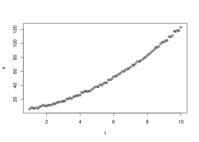
Let us generate some artificial data with the classical formula for uniformly accelerated movement, \(s(t) = s_0 + v_0t + \frac{1}{2}at^2\):
library(quantities)
set.seed(1234)

t <- seq(1, 10, 0.1)
s <- 3 + 2*t + t^2

# some noise added
df <- data.frame(
  t = set_quantities(t + rnorm(length(t), 0, 0.01), s, 0.01),
  s = set_quantities(s + rnorm(length(t), 0, 1), m, 1)
)
plot(df)
Then, we try to adjust a linear model using lm:
fit <- lm(s ~ poly(t, 2), df) # error Ops.units
## Error in Ops.units(X, Y, ...): power operation only allowed with length-one numeric power
First issue: it seems that poly computes powers in a vectorised way
(i.e., t^0L:degree), which is not currently supported in units,
because it would generate different units for each value. Now that
mixed units are supported, this could be a way to circumvent this, but
it is not clear whether the resulting list of mixed units may create
more problems. This is something that we should explore anyway.
Let us try this time by explicitly defining the powers:
(fit <- lm(s ~ t + I(t^2), df))
## Warning: In 'Ops' : non-'errors' operand automatically coerced to an
## 'errors' object with no uncertainty

##
## Call:
## lm(formula = s ~ t + I(t^2), data = df)
##
## Coefficients:
## (Intercept)            t       I(t^2)
##       3.373        1.910        1.006
Now it works. We obtain the (unitless, errorless) coefficients, and these are other parameters and summaries:
coef(fit) # plain numeric, as show above
## (Intercept)           t      I(t^2)
##    3.373459    1.909901    1.006140
residuals(fit)[1:5] # wrong uncertainty, copied from 's'
## Units: [m]
## Errors: 1 1 1 1 1
##           1           2           3           4           5
##  0.01289180  1.41273622  0.68031389 -0.65668199  0.07589058
fitted(fit)[1:5] # wrong uncertainty
## Units: [m]
## Errors: 0 0 0 0 0
##        1        2        3        4        5
## 6.242304 6.703228 7.161199 7.451099 8.039660
predict(fit, data.frame(t=11:15)) # plain numeric
##        1        2        3        4        5
## 146.1253 171.1765 198.2399 227.3156 258.4035
summary(fit) # error Ops.units
## Error in Ops.units(mean(f)^2, var(f)): both operands of the expression should be "units" objects
In summary, we do not get the benefit of obtaining coefficients, fitted values, predictions… with the right units and uncertainty, and the whole object is a mess due to diverse incompatibilities.
Wrapping linear models
There are several possible ways to overcome the issues above. The most
direct one would be to wrap the lm call, so that quantities are
dropped before calling lm, and the resulting object is modified to set
up the proper quantities a posteriori. However, in this way, some
lm methods may work while some others may still be broken.
A cleaner approach would be to wrap the lm call to add a custom class
to the hierarchy and save units and errors for later use:
qlm <- function(formula, data, ...) {
  # get units info, then drop quantities
  row <- data[1,]
  for (var in colnames(data)) if (inherits(data[[var]], "quantities")) {
    data[[var]] <- drop_quantities(data[[var]])
  }

  # fit linear model and add units info for later use
  fit <- lm(formula, data, ...)
  fit$units <- lapply(eval(attr(fit$terms, "variables"), row), units)
  class(fit) <- c("qlm", class(fit))
  fit
}

(fit <- qlm(s ~ t + I(t^2), df))
##
## Call:
## lm(formula = formula, data = data)
##
## Coefficients:
## (Intercept)            t       I(t^2)
##       3.373        1.910        1.006
class(fit)
## [1] "qlm" "lm"
Then, this custom class can be used to build specific methods of interest:
coef.qlm <- function(object, ...) {
  # compute coefficients' units
  coef.units <- lapply(object$units, as_units)
  for (i in seq_len(length(coef.units)-1)+1)
    coef.units[[i]] <- coef.units[[1]]/coef.units[[i]]
  coef.units <- lapply(coef.units, units)

  # use units above and vcov diagonal to set quantities
  coef <- mapply(set_quantities, NextMethod(), coef.units,
                 sqrt(diag(vcov(object))), mode="symbolic", SIMPLIFY=FALSE)

  # use the rest of the vcov to set correlations
  p <- combn(names(coef), 2)
  for (i in seq_len(ncol(p)))
    covar(coef[[p[1, i]]], coef[[p[2, i]]]) <- vcov(fit)[p[1, i], p[2, i]]

  coef
}

coef(fit)
## $`(Intercept)`
## 3.4(5) [m]
##
## $t
## 1.9(2) [m/s]
##
## $`I(t^2)`
## 1.01(2) [m/s^2]
fitted.qlm <- function(object, ...) {
  # set residuals as std. errors of fitted values
  set_quantities(NextMethod(), object$units[[1]],
                 residuals(object), mode="symbolic")
}

fitted(fit)[1:5]
## Units: [m]
## Errors: 0.01289180 1.41273622 0.68031389 0.65668199 0.07589058
##        1        2        3        4        5
## 6.242304 6.703228 7.161199 7.451099 8.039660
predict.qlm <- function(object, ...) {
  # set se.fit as std. errors of predictions
  set_quantities(NextMethod(), object$units[[1]],
                 NextMethod(se.fit=TRUE)$se.fit, mode="symbolic")
}

predict(fit, data.frame(t=11:15))
## Units: [m]
## Errors: 0.4570381 0.6507279 0.8804014 1.1448265 1.4434174
##        1        2        3        4        5
## 146.1253 171.1765 198.2399 227.3156 258.4035
and so on and so forth.
Open problems
This analysis is limited to the lm function, but there are others,
both in R base (such as glm) and in other packages, which have
different sets of input parameters and output. Instead of developing
multiple sets of wrappers and methods, it would be desirable to manage
everything through a common wrapper, class and set of methods (see,
e.g., how ggplot2::geom_smooth works). It should be assessed whether
this is possible, at least for a limited, widely-used, group of
functions.
Also, there may be users interested in fitting linear models with units only, or with uncertainty only. As with the rest of the functionalities in these packages, it should be studied how to wisely break down this feature.
Summary
This article summarises the latest enhancements in the units, errors
and quantities packages, and provides some initial prospects on
fitting linear models with quantities. Also, this is the last
deliverable of the R-quantities project, which has reached the following
milestones:
- A first working prototype.
- Support for units and errors parsing.
- An analysis of data wrangling operations with quantities.
- Prospects on fitting linear models with quantities.
And along the way, there have been multiple exciting improvements, both
in units and errors, to support all these features and make
quantities possible, which is ready for an imminent CRAN release. This
project ends, but the r-quantities
GitHub organisation will continue to thrive and to provide the best
tools for quantity calculus to the R community.
Acknowledgements
This project gratefully acknowledges financial support from the R Consortium. Also I would like to thank Edzer Pebesma for his continued support and collaboration.