Using stars for remote big Earth Observation data processing
- Summary
- The data
- Server
- Client
- Query data
- Process:
st_apply, NDVI - Limitations and lessons learned
- Try this at home
- The way forward
- Earlier stars blogs
Summary
This is the third blog on the
stars project, an R-Consortium
funded project for spatiotemporal tidy arrays with R. It shows how
stars can be used in a client/server setup, where large amounts of
Earth observation data are held on a server, and an (R) client is used
to query the data, process it on the server side, and retrieve a
(small) portion, for example to plot.
This blog is a proof of concept, and was developed for the use case of
remotely processing a set of Sentinel
2 images; no serious effort
has been made so far to generalize this to other image sources. We use the
stars package both on server and client side.
The data
Our dataset consists of 36 zip files, containing Sentinel
2 scenes (or images, tiles,
granules). Together they are 20 Gb. GDAL has a
driver for such zip files, and
hence stars can read them directly. Each zip file contains over 100
files, of which 15 are JPEG2000 files with imagery having 10, 20 or 60 m
resolution. We focus on the 10 m bands (Red, Green, Blue, Near
Infrared); single images of these have 10980 x 10980 pixels, but also
come with overview (downsampled) levels fo 20, 40, 80 and 160 m. That is
convenient, because for plotting it does not make much sense to
transport more pixels than our screen has.
The data were downloaded from ESA’s
SciHub, which first looks cumbersome
but in the end it was quite easy using aria2c. (The aria2 file
contains my user credentials.)
Server
The server side is set up using plumber:
library(plumber)
r <- plumb("server.R")
r$run(port=8000)
The server.R script is now explained in sections.
Reading data
The following script reads all the files ending in .zip, and creates
names from them that are understood by the GDAL Sentinel 2
driver. The /vsizip prefix
makes sure that the zip files is read as if it were unzipped. Function
read_stars_meta reads as much as possible metadata from the set of
files (and their subdatasets: here only subdataset 1, which has the 10 m
x 10 m imagery), and returns it in a (still) somewhat chaotic nested
list. The object md is an sf-tibble with names and bounding boxes (as
polygon feature geometries) of every image.
library(jsonlite) # base64_enc
library(stars)
library(tibble)

# load some imagery meta data
# from a S2 .zip file, create a readable gdal source:
s2_expand_zip = function(s) {
    paste0("/vsizip/", s, "/", sub(".zip", ".SAFE", s), "/MTD_MSIL1C.xml")
}
lst = list.files(pattern = "*.zip")
l = lapply(s2_expand_zip(lst), read_stars_meta, sub = 1)
bb <- do.call(c, lapply(l, function(x) st_as_sfc(st_bbox(st_dimensions(x)))))
fn = sapply(l, function(x) attr(x, "file_names"))
md = st_sf(tibble(file = fn, geom = bb))

# global database
data = list(md = md)
Serving /data
The following function simply logs every request to screen and forwards it:
#* Log some information about the incoming request
#* @filter logger
function(req){
  cat(as.character(Sys.time()), "-",
    req$REQUEST_METHOD, req$PATH_INFO, "-",
    req$HTTP_USER_AGENT, "@", req$REMOTE_ADDR, ":", req$postBody, "\n")
  plumber::forward()
}
The final two functions do the real work: they read an expression, evaluate it and return the result (get), or they store the result on the server side (put):
# plumber REST end points /data:
#* @get  /data
#* @post /data
get_data <- function(req, expr = NULL) {
    print(expr)
    if (is.null(expr))
        names(data)
    else
        base64_enc(serialize( eval(parse(text = expr), data), NULL)) # to char
}

#* @put /data
put_data <- function(req, name, value) {
    data[[name]] <<- unserialize(base64_dec(fromJSON(value)))
    NULL
}
This means that GET http://x.y/data gives a listing of available
datasets, and GET http://x.y/data/obj retrieves object obj. PUT
uploads objects to the database (called data).
Client
On the client side, we need to also do some work:
I/O with the server:
library(httr)     # GET, POST, PUT
library(jsonlite) # base64_dec, base64_enc, toJSON, fromJSON
## Loading required package: methods

get_data = function(url, expr = NULL) {
    if (is.null(expr))
        fromJSON( content(GET(url), "text", encoding = "UTF-8"))
    else
        unserialize(base64_dec(fromJSON(
            content(POST(url, body = list(expr = expr), encode = "json"),
                "text", encoding = "UTF-8")
        )))
}

put_data = function(url, name, value) {
    value = toJSON(base64_enc(serialize(value, NULL)))
    PUT(url, body = list(name = name, value = value), encode = "json")
}
Somewhat confusingly I gave these the same name as on the server side,
but these exist in a different R session: the one you interact with
directly, the client. For get_data, the return value is decoded and
unserialized to get a copy of the original R object on the server. This
R object may have been present at the server, or may have been created
on the server: since the server uses eval, it takes arbitrary R
expressions.
Example client session: metadata
We can get a view of the data present on the server by
url = "http://localhost:8000/data"
get_data(url) # list
## [1] "md"
Next, we can retrieve the md (metadata) object:
library(stars)
## Loading required package: abind
## Loading required package: sf
## Linking to GEOS 3.5.1, GDAL 2.2.1, proj.4 4.9.3
library(tibble)   # print
md = get_data(url, "md")
md
## Simple feature collection with 36 features and 1 field
## geometry type:  POLYGON
## dimension:      XY
## bbox:           xmin: 3e+05 ymin: 5590200 xmax: 809760 ymax: 6e+06
## epsg (SRID):    32631
## proj4string:    +proj=utm +zone=31 +datum=WGS84 +units=m +no_defs
## # A tibble: 36 x 2
##    file                                                               geom
##    <chr>                                                     <POLYGON [m]>
##  1 SENTINEL2_L1C:/vsizip/S2A_MSIL1C_20… ((499980 5890200, 609780 5890200,…
##  2 SENTINEL2_L1C:/vsizip/S2A_MSIL1C_20… ((6e+05 5890200, 709800 5890200, …
##  3 SENTINEL2_L1C:/vsizip/S2A_MSIL1C_20… ((699960 5690220, 809760 5690220,…
##  4 SENTINEL2_L1C:/vsizip/S2A_MSIL1C_20… ((3e+05 5690220, 409800 5690220, …
##  5 SENTINEL2_L1C:/vsizip/S2A_MSIL1C_20… ((499980 5590200, 609780 5590200,…
##  6 SENTINEL2_L1C:/vsizip/S2A_MSIL1C_20… ((6e+05 5590200, 709800 5590200, …
##  7 SENTINEL2_L1C:/vsizip/S2A_MSIL1C_20… ((6e+05 5690220, 709800 5690220, …
##  8 SENTINEL2_L1C:/vsizip/S2A_MSIL1C_20… ((6e+05 5790240, 709800 5790240, …
##  9 SENTINEL2_L1C:/vsizip/S2A_MSIL1C_20… ((6e+05 5890200, 709800 5890200, …
## 10 SENTINEL2_L1C:/vsizip/S2A_MSIL1C_20… ((699960 5590200, 809760 5590200,…
## # ... with 26 more rows
Query data
We will now create an RGB mosaic of the data, while reading them at overview level 3, meaning 160 m x 160 m pixels.
# select a country:
nl = st_as_sf(raster::getData("GADM", country = "NLD", level = 0)) %>%
    st_transform(st_crs(md))

file = md[nl,]$file
plot(st_geometry(nl), axes = TRUE)
s = sapply(file, function(x) {
    expr = paste0("read_stars(\"", x, "\", options = \"OVERVIEW_LEVEL=3\", NA_value = 0)")
    r = get_data(url, expr)
    image(r, add = TRUE, rgb = 4:2, maxColorValue = 15000)
})
plot(st_geometry(md), border = 'yellow', add = TRUE, lwd = .8)
plot(st_geometry(nl), add=TRUE, border = 'orange', lwd = 2)
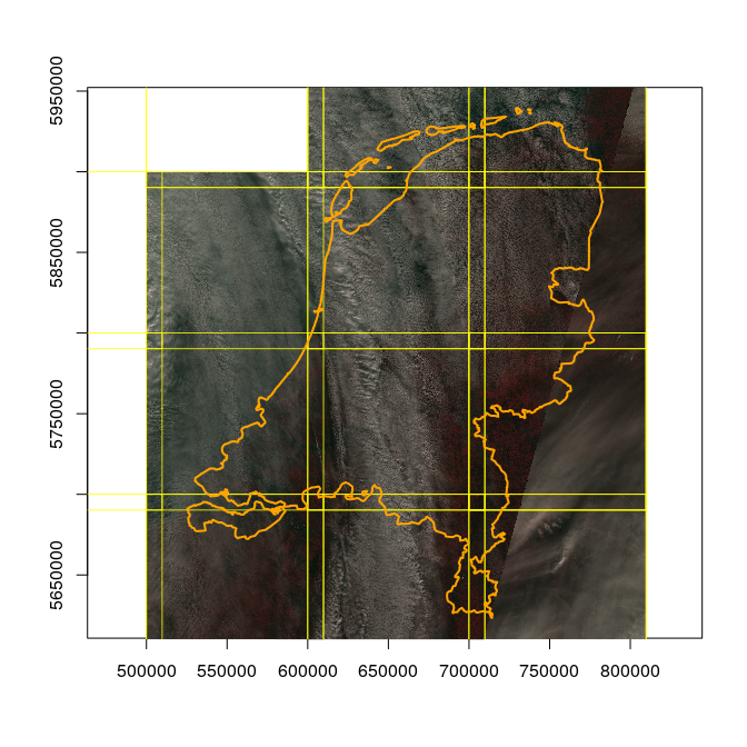
The expression file = md[nl,]$file selects the file names from the
image metadata md for those scenes (images) that intersect with the
country (nl).
On top of the image (which shows mostly clouds) we plotted the country boundary, and the tile boundaries.
Process: st_apply, NDVI
This way, we can also create new variables on the server side and show
them. As an example, we can use st_apply which does an apply to the arrays
in a stars object (and takes care of the dimensions afterwards!), and
define an
NDVI
function, which we upload to the server:
ndvi = function(x) (x[4]-x[1])/(x[4]+x[1])
put_data(url, "ndvi", ndvi)
## Response [http://localhost:8000/data]
##   Date: 2018-03-23 03:01
##   Status: 200
##   Content-Type: application/json
##   Size: 2 B
get_data(url)
## [1] "md"   "ndvi"
get_data(url, "ndvi")
## function(x) (x[4]-x[1])/(x[4]+x[1])
Next, we can query the server giving it an expression that applies the ndvi function to the (overview level 3) imagery, and returns the single-band (NDVI) image:
plot(st_geometry(nl), axes = TRUE)
s = sapply(file, function(x) {
    expr = paste0("st_apply(read_stars(\"", x, "\", options = \"OVERVIEW_LEVEL=3\", NA_value = 0),
        1:2, ndvi)")
    r = get_data(url, expr)
    image(r, add = TRUE, zlim = c(-1,1), col = colorRampPalette(c(grey(.1), grey(.5), 'green'))(10))
})
plot(st_geometry(nl), add = TRUE) # once more
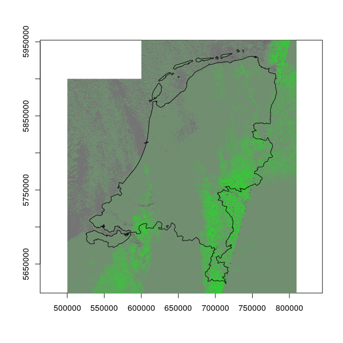
The diagonal line is caused by the fact that we combine imagery from different satellite overpasses, of which most are pretty cloudy.
Computing NDVI is just one example; the Index database contains 200 more indexes that can be computed from Sentinel 2 data.
Limitations and lessons learned
- As a prototype, this implementation has strong limitations. To use this in an architecture with multiple, concurrent users would require authentication, user management, and concurrent R sessions.
- if we try to read one full 10 m scene with 4 bands from the server,
we see the error
long vectors not supported, indicating that the encoded data is over 2 Gb; file download and upload will be needed for larger data sizes, or more clever interaction patterns such as a web map service or tile map service. - to pass R objects, we need to
serializethem,base64_encthat, and wrap the result intoJSON. On the receiver side, we need to do the reverse (fromJSON,base_64_dec,unserialize). - never try to put an R expression or its base64 encoding in a url
(using
GET) - usePOSTand put it in the message body;GETwill do funny things with funny characters (even=). - the way we submit expressions looks pretty messy using character strings, there must be a more tidy way to do this.
Try this at home
No blog without a reproducible example! Start two R sessions, one for a client, one for a server. On the server sessions, run:
devtools::install_github("stars") # requires sf 0.6-1, which is now on CRAN
library(plumber)
r <- plumb(system.file("plumber/server.R", package = "stars"))
r$run(port=8000)
and keep this running! On the client session, run
source(system.file("plumber/client.R", package = "stars"),, echo = TRUE)
and watch for the logs from the server. In the client, you can now
plot(xx)
to see an object that was read in the server session.
The way forward
Where this example worked locally, and thus automatically with “small” large data (20 Gb imagery), in next steps we will develop and deploy this with “large” large data. Amazon hosts large collections of Landsat 8 and Sentinel 2 L1C data, and with the setup sketched above it should be fairly straightforward to directly compute on these data, given access to a cloud back-end machine. The R Consortium has sponsored the Earth data processing backend for testing and evaluating stars project, which has a budget for a storage and/or compute back-end for evaluation purposes.
openEO is a project that develops an open API to connect R, python and javascript clients to big Earth observation cloud back-ends in a simple and unified way. That is a similar ambition, but larger. openEO uses a process graph (directed, acyclic graph) to represent the expression, which must be acceptable for all back-ends. Here, we have R on both sides of the wire, which makes life much more simple. But openEO is also a cool project: check out the proof of concept videos!