Plotting and subsetting stars objects

Summary
Plots of raster data
Subsetting
Conversions: raster, spacetime
Easier set-up
Earlier stars blogs

Summary

This is the second blog on the stars project, an R-Consortium funded project for spatiotemporal tidy arrays with R. It shows how stars plots look (now), how subsetting works, and how conversion to Raster and ST (spacetime) objects works.

I will try to make up for the lack of figures in the last two r-spatial blogs!

Plots of raster data

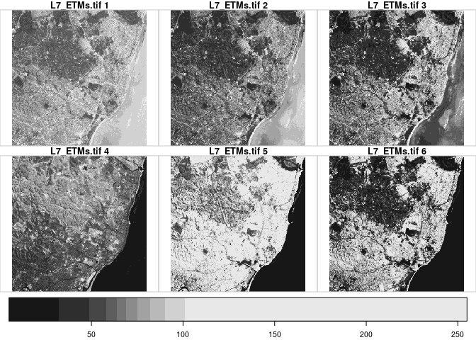
We’ve become accustomed to using the raster package for plotting raster data, as in:

library(raster)
## Loading required package: methods
## Loading required package: sp
tif = system.file("tif/L7_ETMs.tif", package = "stars")
(r = stack(tif))
## class       : RasterStack 
## dimensions  : 352, 349, 122848, 6  (nrow, ncol, ncell, nlayers)
## resolution  : 28.5, 28.5  (x, y)
## extent      : 288776.3, 298722.8, 9110729, 9120761  (xmin, xmax, ymin, ymax)
## coord. ref. : +proj=utm +zone=25 +south +ellps=GRS80 +towgs84=0,0,0,0,0,0,0 +units=m +no_defs 
## names       : L7_ETMs.1, L7_ETMs.2, L7_ETMs.3, L7_ETMs.4, L7_ETMs.5, L7_ETMs.6 
## min values  :         0,         0,         0,         0,         0,         0 
## max values  :       255,       255,       255,       255,       255,       255
plot(r)

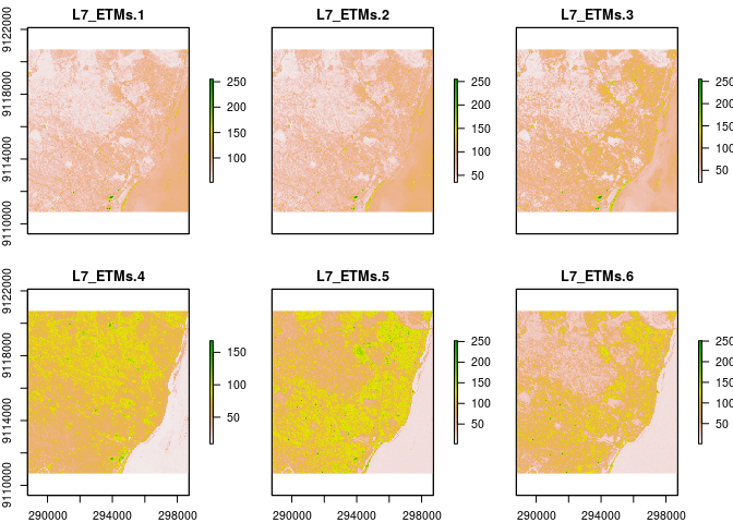
stars does a similar layout, but chooses quite a few different defaults:

library(stars)
## Loading required package: abind
## Loading required package: sf
## Linking to GEOS 3.5.1, GDAL 2.2.1, proj.4 4.9.3
(x = read_stars(tif))
## stars object with 3 dimensions and 1 attribute
## attribute(s):
##   L7_ETMs.tif    
##  Min.   :  1.00  
##  1st Qu.: 54.00  
##  Median : 69.00  
##  Mean   : 68.91  
##  3rd Qu.: 86.00  
##  Max.   :255.00  
## dimension(s):
##      from  to  offset delta                       refsys point values
## x       1 349  288776  28.5 +proj=utm +zone=25 +south... FALSE   NULL
## y       1 352 9120761 -28.5 +proj=utm +zone=25 +south... FALSE   NULL
## band    1   6      NA    NA                           NA    NA   NULL
plot(x)

The defaults include:

the plots receive a joint legend, rather than a legend for each layer; where raster considers the bands as independent layers, stars treats them as a single variable that varies over the dimension band;
the plot layout (rows \(\times\) columns) is chosen such that the plotting space is filled maximally with sub-plots;
a legend is placed on the side where the most white space was left;
color breaks are chosen by classInt::classIntervals using the quantile method, to get maximum spread of colors;
a grey color pallete is used;
grey lines separate the sub-plots.

Optimisations that were implemented to avoid long plotting times include:

the data is subsampled to a resolution such that not substantially more array values are plotted than the pixels available on the plotting device (dev.size("px"));
the quantiles are computed from maximally 10000 values, regularly sampled from the array.

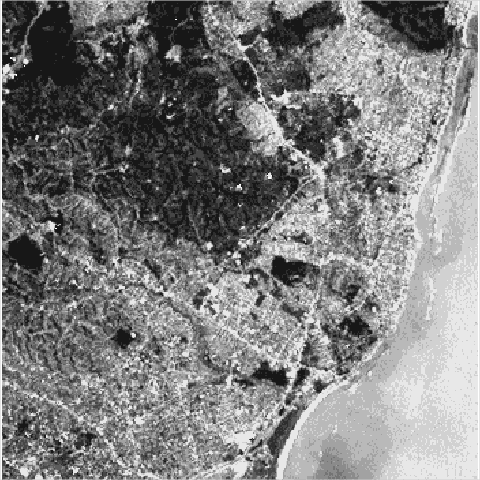
If we want to maximize space, a space-filling plot for band 1 is obtained by

plot(x[,,,1], main = NULL, key.pos = NULL)

A more dense example with climate data, which came up here, looks like this:

Tim has done some cool experiments with plotting stars objects with mapview, and interacting with them - that will have to be a subject of a follow-up blog post.

Subsetting

This brings us to subsetting! stars objects are collections (lists) of R arrays with a dimension (metadata, array labels) table in the attributes. R arrays have a powerful subsetting mechanism with [, e.g. where x[,,10,] takes the 10-th slice along the third dimension of a four-dimensional array. I wanted a [ method for my own class, which has an arbitrary number of dimensions, but using [.array. I tried it with base R, as well as with rlang. Both are a bit of an adventure, you essentially build your custom call, and then call it. Hadley Wickham’s Advanced R book helped a lot!

Anyway, we can now, as we saw, subset stars objects by

x[,,,1]
## stars object with 3 dimensions and 1 attribute
## attribute(s):
##   L7_ETMs.tif    
##  Min.   : 47.00  
##  1st Qu.: 67.00  
##  Median : 78.00  
##  Mean   : 79.15  
##  3rd Qu.: 89.00  
##  Max.   :255.00  
## dimension(s):
##      from  to  offset delta                       refsys point values
## x       1 349  288776  28.5 +proj=utm +zone=25 +south... FALSE   NULL
## y       1 352 9120761 -28.5 +proj=utm +zone=25 +south... FALSE   NULL
## band    1   1      NA    NA                           NA    NA   NULL

but hey, this was a three-dimensional array, right? Indeed, but we may also want to select the array in question (stars objects are a list of arrays), and this is done with the first index.

In addition to this, we can crop an image by using a polygon as first index. For instance, by taking a circle around the centroid of the image:

pol <- x %>% st_bbox() %>% st_as_sfc() %>% st_centroid() %>% st_buffer(300)
x <- x[,,,1]
plot(x[pol])

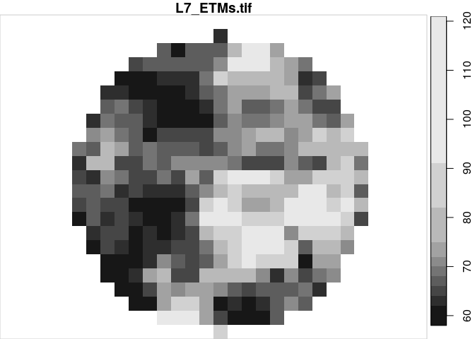This creates a circular “clip”; in practice, the grid is cropped (or cut back) to the bounding box of the circular polygon, and values outside the polygon are assigned NA values.

Doing all this with filter (for dimensions) and select (for arrays) is next on my list.

Conversions: raster, spacetime

A round-trip through Raster (in-memory!) is shown for the L7 dataset:

library(raster)
(x.r = as(x, "Raster"))
## class       : RasterBrick 
## dimensions  : 352, 349, 122848, 1  (nrow, ncol, ncell, nlayers)
## resolution  : 28.5, 28.5  (x, y)
## extent      : 288776.3, 298722.8, 9110729, 9120761  (xmin, xmax, ymin, ymax)
## coord. ref. : +proj=utm +zone=25 +south +ellps=GRS80 +towgs84=0,0,0,0,0,0,0 +units=m +no_defs 
## data source : in memory
## names       : layer 
## min values  :    47 
## max values  :   255 
## time        : NA
st_as_stars(x.r)
## stars object with 3 dimensions and 1 attribute
## attribute(s):
##                  
##  Min.   : 47.00  
##  1st Qu.: 67.00  
##  Median : 78.00  
##  Mean   : 79.15  
##  3rd Qu.: 89.00  
##  Max.   :255.00  
## dimension(s):
##      from  to  offset delta                       refsys point values
## x       1 349  288776  28.5 +proj=utm +zone=25 +south...    NA   NULL
## y       1 352 9120761 -28.5 +proj=utm +zone=25 +south...    NA   NULL
## band    1   1      NA    NA                           NA    NA     NA

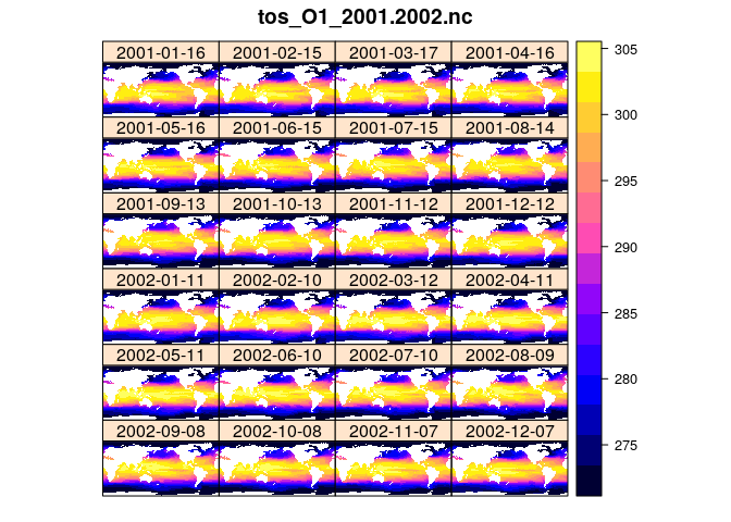
A round-trip through spacetime is e.g. done with an example NetCDF file (it needs to have time!):

library(stars)
nc = read_stars(system.file("nc/tos_O1_2001-2002.nc", package = "stars"))
plot(nc)

s = as(nc, "STFDF")
library(spacetime)
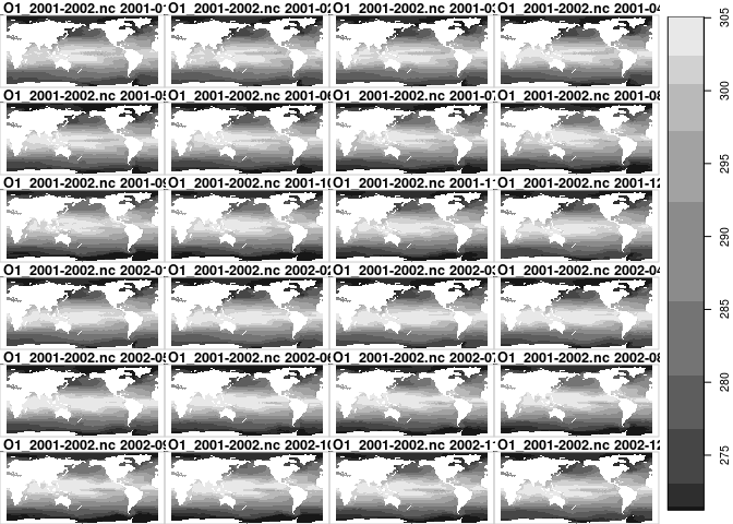
stplot(s) # uses lattice!

This has flattened 2-D space to 1-dimensional set of features (SpatialPixels):

dim(s)
##     space      time variables 
##     30600        24         1
s[1, 1, drop = FALSE]
## An object of class "STFDF"
## Slot "data":
##   tos_O1_2001.2002.nc
## 1            271.4592
## 
## Slot "sp":
## Object of class SpatialPixels
## Grid topology:
##           cellcentre.offset cellsize cells.dim
## coords.x1               1.0        2       180
## coords.x2             -79.5        1       170
## SpatialPoints:
##   coords.x1 coords.x2
## 1         1      89.5
## Coordinate Reference System (CRS) arguments: NA 
## 
## Slot "time":
## Warning: timezone of object (UTC) is different than current timezone ().
##            ..1
## 2001-01-16   1
## 
## Slot "endTime":
## [1] "2001-02-15 UTC"

Easier set-up

I decided to move all code in stars that depends on the GDAL library to package sf. This not only makes maintainance lighter (both for me and for CRAN), but also makes stars easier to install, e.g. using devtools::install_github. Also, binary installs will no longer require to have two local copies of the complete GDAL library (and everything it links to) on every machine.

Earlier stars blogs

first stars blog