In r-spatial, the Earth is no longer flat
sfup to 0.9-x uses mostly a flat Earth modelsf1.0: Goodbye flat Earth, welcome S2 spherical geometry- Where did the ellipsoid go?
- Where did my equirectangular logic go?
- How to test this?
- What is next?
Summary: Package sf is undergoing a major change: all operations
on geographical coordinates (degrees longitude, latitude) will use the
s2 package, which interfaces the S2 geometry library for spherical
geometry.
sf up to 0.9-x uses mostly a flat Earth model
Suppose you work with package sf, have loaded some data
library(sf)

## Linking to GEOS 3.8.0, GDAL 3.0.4, PROJ 7.0.0

nc = read_sf(system.file("gpkg/nc.gpkg", package="sf"))
then chances are large that after running e.g.
i = st_intersects(nc)
you’ve run into the following message
## although coordinates are longitude/latitude, st_intersects assumes that they are planar
It indicates that
- your data are in geographical coordinates, degrees longitude/latitude indicating a position on the globe, and
- you are carrying out an operation that assumes these data lie in a flat plane, where one degree longitude equals one degree latitude, irrespective where you are on the world
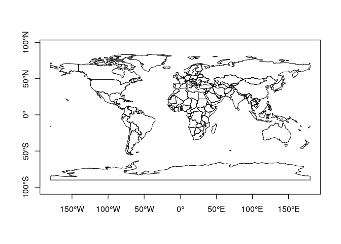
This means that your data are assumed implicitly to be projected to the equirectangular projection, looking like this:
library(rnaturalearth)
ne <- countries110 %>%
  st_as_sf() %>%
  st_geometry()
plot(ne, axes = TRUE)
A number of operations in sf were actually carried out using
ellipsoidal geometries, these included
- computing the area of polygons, which used
lwgeom::st_geod_area - computing length of lines, which used
lwgeom::st_geod_length - computing distance between features, which used
lwgeom::st_geod_distance, and - segmentizing lines along great circles, which used
lwgeom::st_geod_segmentize
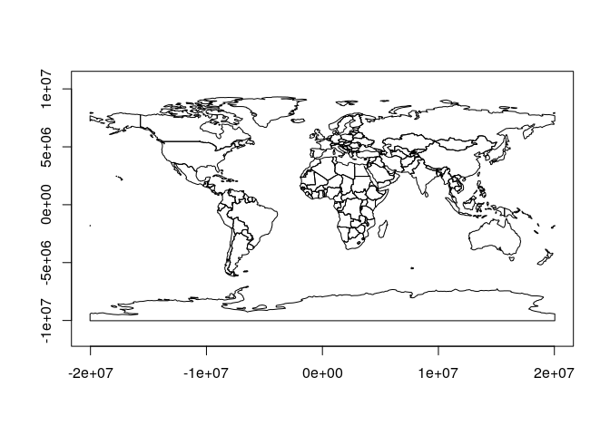
but for all other operations, despite the degree symbols, everything happens just as if they were in the equivalent equirectangular projection:
st_transform(ne, "+proj=eqc") %>%
  plot(axes = TRUE)
As an example, consider the polygon from
POLYGON((-150 -65, 0 -62, 120 -78, -150 -65)), drawn as a line in this
projection 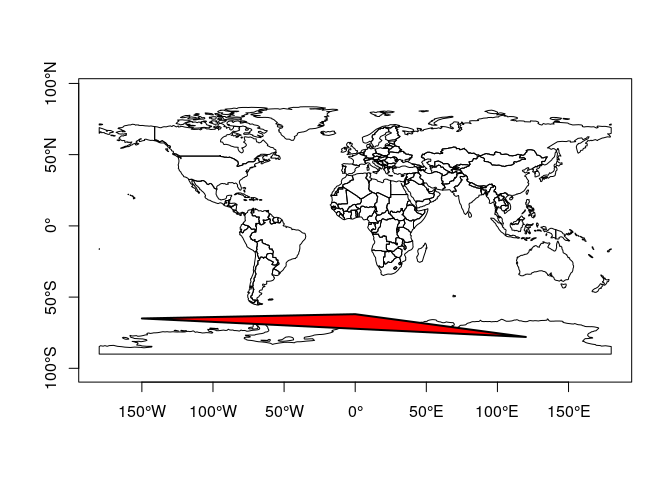
corresponds to this polygon when drawn in a stereographic polar
projection: 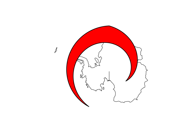
and does not include the South Pole:
pol = st_as_sfc("POLYGON((-150 -65, 0 -62, 120 -78, -150 -65))")
pole = st_as_sfc("POINT(0 -90)")
st_contains(pol, pole)

## Sparse geometry binary predicate list of length 1, where the predicate was `contains'
##  1: (empty)
(with sf 0.9-x, setting crs to 4326 will have no effect other than
printing the familiar warning message)
The functions in sf up to 0.9-x that assume a flat Earth include:
- all binary predicates (
intersects,touches,covers,contains,equals,equals_exact,relate, …) - all geometry generating operators (
centroid,intersection,union,difference,sym_difference) st_sample- nearest functions:
nearest_point,nearest_feature - functions or methods using these:
st_filter,st_join,agreggate,[, …
In addition to this, a number of ugly “hacks” needed to make things work include:
- polygons and lines crossing the antimeridian (longitude +/- 180) had
to be cut in two, using
sf::st_wrap_dateline - polygons containing e.g. the South Pole needed to pass through (-180,-90) and (180,90)
- raster data with longitude ranging from 0 to 360 could not be properly combined with -180,180 data
- for orthographic projections (Earth seen from space, or “spinning globes”), selecting countries on the “visible” half of the Earth was very ugly
sf 1.0: Goodbye flat Earth, welcome S2 spherical geometry
From version 1.0 on, wherever possible, when handling geographic
coordinates package sf uses the S2 geometry
library for spatial operations. This library was written by Google, and
empowers critical parts of Google Earth, Google Maps, Google Earth
Engine and Google Bigquery GIS. The s2 R
package is a complete rewrite of the
original s2 package by Ege Rubak (still on CRAN), mostly done by Dewey
Dunnington and Edzer Pebesma.
S2 geometry assumes that straight lines between points on the globe are
not formed by straight lines in the equirectangular projection, but by
great circles: the shortest path over the sphere. For the polygon above
this would give: 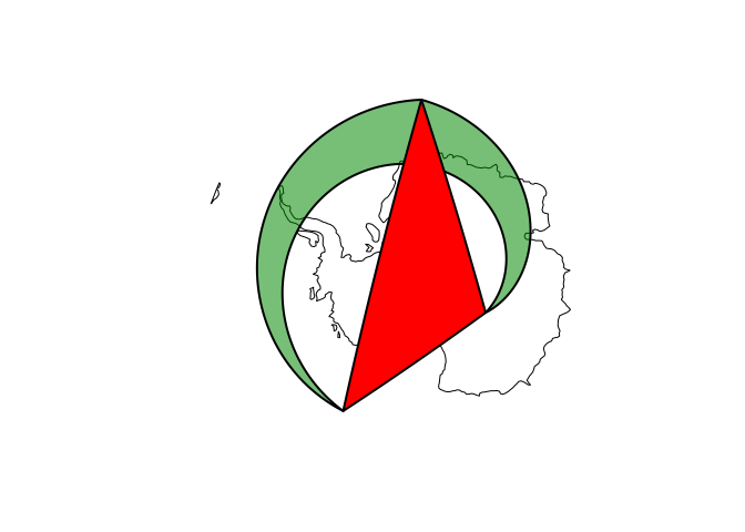
where the light green polygon is the “straight line polygon” in equirectangular. Based on the great circle lines, this polygon now contains the South Pole:
pol = st_as_sfc("POLYGON((-150 -65, 0 -62, 120 -78, -150 -65))", crs = 4326)
pole = st_as_sfc("POINT(0 -90)", crs = 4326)
st_contains(pol, pole)

## Sparse geometry binary predicate list of length 1, where the predicate was `contains'
##  1: 1
Where did the ellipsoid go?
Although we know that an ellipsoid better approximates the Earths’
shape, computations done with s2 are all on a spere. The ellipsoidal
functions in package lwgeom (lwgeom::st_geod_area,
lwgeom::st_geod_length, lwgeom::st_geod_distance, and
lwgeom::st_geod_segmentize) can, for now, still be called when setting
argument use_lwgeom=TRUE to sf::st_area() etc., but in order to
reduce the complexity of maintaining dependencies of package sf this
will most likely be deprecated, in which case users will have to call
these functions directly when needed.
The difference between ellipsoidal and spherical computations is roughly up to 0.5%; here, for areas it is
units::set_units(1) - mean(st_area(nc) / st_area(nc, use_lwgeom = TRUE)) # difference to ellipsoidal

## 6.446441e-05 [1]
In calls to s2 measures, the radius of the Earth can be specified:
st_area(nc[1,]) # default radius: 6371010 m

## 1137107793 [m^2]

st_area(nc[1,], radius = units::set_units(1, m)) # unit sphere

## 2.801464e-05 [m^2]
Where did my equirectangular logic go?
You can always get back the old behaviour by projecting your geographic coordinates to the equirectangular projection, and working from there, e.g. by
nc = st_transform(nc, "+proj=eqc")
How to test this?
The new s2 package can be installed by
remotes::install_github("r-spatial/s2")
For sf support, as shown above, you now need to install the s2
branch:
remotes::install_github("r-spatial/sf", ref = "s2")
Please report back any experiences!
What is next?
This is all part of the R-global R Consortium ISC project, the proposal of which can be found here. Actually using the S2 library is new to us, and we still need to learn much more about
- how to use the S2 library effectively
- what is faster, what is slower than e.g. GEOS, and why
- how to effectively use the S2 indexing structures
In follow-up blog posts we will elaborate on
- differences between geometrical operations in the flat plane and on the sphere
- special features of the S2 library: S2Cells, S2Caps, the full polygon, the virtue of half-open polygons, …
- how all this can be beneficial for spatial analysis, and e.g. with handling raster data