Parallel raster processing in stars
Summary:
Prediction on large datasets can be time-consuming, but with enough
computing power, this task can be parallelized easily. Some algorithms
provide native multithreading like predict() function in the
{ranger} package (but this is not standard). In this situation, we
have to parallelize the calculations ourselves. There are several
approaches to do this, but for this example we will divide a large out
of memory raster into smaller blocks and make predictions using
multiprocessing.
Data acquisition
We will use the Landsat 8 satellite scene with four spectral bands as an example for analysis. It covers a range of 37,000 km2 and consists of over 62 million pixels. The data is available on Zenodo.
We can use the download.file() function to download the data and then
unpack the .zip archive using the unzip() function.
options(timeout = 600) # increase connection timeout
url = "https://zenodo.org/record/8260938/files/Landsat.zip"
download.file(url, "Landsat.zip")
unzip("Landsat.zip")
Data loading
library("stars")
set.seed(1) # define a random seed
The first step is to list the rasters representing the blue (B2), green
(B3), red (B4), and near infrared (B5) bands to be loaded using the
list.files() function. We need to define two additional arguments,
i.e. pattern = "\\.TIF$" and full.names = TRUE.
files = list.files("Landsat", pattern = "\\.TIF$", full.names = TRUE)
files

## [1] "Landsat/LC08_L2SP_191023_20230605_20230613_02_T1_SR_B2.TIF"
## [2] "Landsat/LC08_L2SP_191023_20230605_20230613_02_T1_SR_B3.TIF"
## [3] "Landsat/LC08_L2SP_191023_20230605_20230613_02_T1_SR_B4.TIF"
## [4] "Landsat/LC08_L2SP_191023_20230605_20230613_02_T1_SR_B5.TIF"
Since this data does not fit in memory, we have to load it as a proxy
(actually, we will only load the metadata describing these rasters). To
do this, we use the read_stars() function with the arguments
proxy = TRUE and along = 3. This second argument will cause the
bands (layers) to be combined into a three-dimensional array:
[longitude, latitude, spectral band].
rasters = read_stars(files, proxy = TRUE, along = 3)
We can replace the default filenames with band names, and rename the third dimension as follows:
bands = c("Blue", "Green", "Red", "NIR")
# rename bands and dimension
rasters = st_set_dimensions(rasters, 3, values = bands, names = "band")
names(rasters) = "Landsat" # rename the object
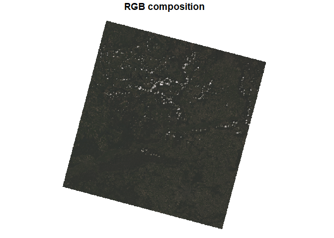
Using the default plot() function, we can display our four bands
separately. By specifying the rgb argument, we can create a three-band
composition, such as RGB or CIR (including near infrared). It is also
useful to use the downsample argument to display the image at a lower
resolution.
plot(rasters, rgb = c(3, 2, 1), downsample = 10, main = "RGB composition")
Sampling
For modeling, we need to use a smaller sample rather than the entire dataset. Sampling training points consists of several steps, which are shown below:
bbox = st_as_sfc(st_bbox(rasters)) # define a bounding box
smp = st_sample(bbox, size = 20000) # sample points from the extent of the polygon
smp = st_extract(rasters, smp) # extract the pixel values for those points
smp = st_drop_geometry(st_as_sf(smp)) # convert to a data frame (remove geometry)
smp = na.omit(smp) # remove missing values (NA)
head(smp)

##   Blue Green   Red   NIR
## 1 9908 11349 11862 19186
## 2 8187  9252  8641 21080
## 3 9377 10576 10837 15875
## 6 9264 10154 10422 13587
## 8 7571  8276  8065 11121
## 9 8090  8799  8162 20219
Modelling
The aim of our analysis is to perform unsupervised classification
(clustering) of raster pixels based on spectral bands. In other words,
we want to group similar cells together to make homogeneous clusters. A
popular method is the Gaussian mixture models available in the
mclust package. Clustering can be done using the Mclust() function
and requires the target number of clusters to be defined in advance
(e.g. G = 6).
library("mclust")
mdl = Mclust(smp, G = 6) # train the model
Prediction
As stated earlier, the entire raster is too large to be loaded into
memory. We need to split it into smaller blocks. For this, we can use
the st_tile() function, which requires the total number of rows and
columns, and the number of rows and columns of a small block (for
example, it could be 2048 x 2048, but usually we should find the optimal
size).
tiles = st_tile(nrow(rasters), ncol(rasters), 2048, 2048)
head(tiles)

##      nXOff nYOff nXSize nYSize
## [1,]     1     1   2048   2048
## [2,]     1  2049   2048   2048
## [3,]     1  4097   2048   2048
## [4,]     1  6145   2048   1807
## [5,]  2049     1   2048   2048
## [6,]  2049  2049   2048   2048
Finally, the input raster will be divided into 16 smaller blocks. In the following sections, we will compare the processing performance of one versus multiple processes.
Now let’s discuss what steps we need to take to make a prediction:
- We have 16 blocks, so we need to make predictions in a loop.
- We have to load the rasters, but this time into memory
(
proxy = FALSE) and only the block (RasterIO = tiles[iterator, ]). - We use the
predict()function for clustering. Note we need to define thedrop_dimensions = TRUEargument to remove the coordinates from the data frame. - Finally, we have to save the clustering results to disk (it can be a
temporary directory). Be sure to specify the missing values
(
NA_value = 0) and the block size as the input (chunk_size = dim(tile)).
Note! The read_stars() function opens the connection to the file
and closes it each time, which causes overhead. With a large number of
blocks, this can significantly affect performance. In this case, it is
better to use a low-level API,
e.g. gdalraster.
The second difference between these packages is that gdalraster
allows loading data stored as integers, while stars loads it as real
(floating point) by default, so we can practically save half of the
memory.
Single process
start_time = Sys.time()

for (i in seq_len(nrow(tiles))) {
  tile = read_stars(files, proxy = FALSE, RasterIO = tiles[i, ])
  names(tile) = bands # rename bands

  pr = predict(tile, mdl, drop_dimensions = TRUE)
  pr = pr[1] # select only clusters from output
  save_path = file.path(tempdir(), paste0("tile_", i, ".tif"))
  write_stars(pr, save_path, NA_value = 0, options = "COMPRESS=NONE",
              type = "Byte", chunk_size = dim(tile))
}

end_time_1 = difftime(Sys.time(), start_time, units = "secs")
end_time_1 = round(end_time_1)
The prediction took 484 seconds.
Multiple processes
Multi-process prediction is a bit more complicated. This requires the
use of two additional packages, i.e. foreach and doParallel. Now
we need to setup a parallel backend by defining the number of available
cores (or by detecting them automatically using detectCores()) in
makeCluster(), and then registering the cluster using the
registerDoParallel() function. This can be accomplished, for instance,
with:
library("foreach")
library("doParallel")
cores = 3 # specify number of cores
cl = makeCluster(cores)
registerDoParallel(cl)
Once we have the computing cluster prepared, we can write a loop that
will be executed in parallel. Instead of the standard for() loop, we
will use foreach() with the %dopar% operator. In foreach() we need
to define an iterator and packages that will be exported to each worker.
Then we use the %dopar% operator and write the core of the function
(is identical to the example using a single process).
packages = c("stars", "mclust")

start_time = Sys.time()

tifs = foreach(i = seq_len(nrow(tiles)), .packages = packages) %dopar% {
  tile = read_stars(files, proxy = FALSE, RasterIO = tiles[i, ], NA_value = 0)
  names(tile) = bands

  pr = predict(tile, mdl, drop_dimensions = TRUE)
  pr = pr[1]
  save_path = file.path(tempdir(), paste0("tile_", i, ".tif"))
  write_stars(pr, save_path, NA_value = 0, options = "COMPRESS=NONE",
              type = "Byte", chunk_size = dim(tile))
  return(save_path)
}

end_time_2 = difftime(Sys.time(), start_time, units = "secs")
end_time_2 = round(end_time_2)
The prediction took 200 seconds. By using three processes instead of one, we have cut the operation time by half!
Post-processing
We have our raster blocks saved in a temporary directory. The final step is to make a mosaic (that is, to combine the blocks into a single raster). I recommend using GDAL tools, as they provide the best performance when there are a large number of blocks. We can use:
buildvrtto create a virtual mosaic.translateto save as a geotiff.
We can call these tools using the gdal_utils() function from the
sf package.
vrt = tempfile(fileext = ".vrt")
gdal_utils(util = "buildvrt", unlist(tifs), destination = vrt)
gdal_utils(util = "translate", vrt, destination = "predict.tif")
Once the parallel computation is complete, we can close the computing
cluster using stopCluster() function (this will delete the temporary
files).
stopCluster(cl)
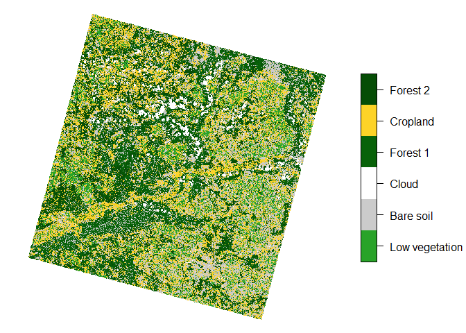
So let’s see what our final map looks like.
clustering = read_stars("predict.tif")
colors = c("#29a329", "#cbcbcb", "#ffffff", "#086209", "#fdd327", "#064d06")
names = c("Low vegetation", "Bare soil", "Cloud", "Forest 1", "Cropland", "Forest 2")
clustering[[1]] = factor(clustering[[1]], labels = names)
plot(clustering, main = NULL, col = colors, key.width = lcm(4))